Intro

In the Spring of 2024 a new LLM evaluation called Humanity’s Last Exam was released. A co-worker sent me the demo page at the time and I found a physics problem relating to a pendulum with a pivot point that slides along the axis. I told him I thought I could solve it (possible I declared I could easily solve it) as a generalization of the pendulum problem taught in physics class years ago. In the process, I revisited the details of the basic pendulum and found that I had actually solved a heinous approximation! Despite its simple seeming setup, the motion of a pendulum is fundamentally complex and resists analytical modeling of its position.

NOTE: The following presumes understanding of single variable calculus, the chain rule, trig functions, trig identities, free body diagrams, and newton’s second law.

Problem Statement

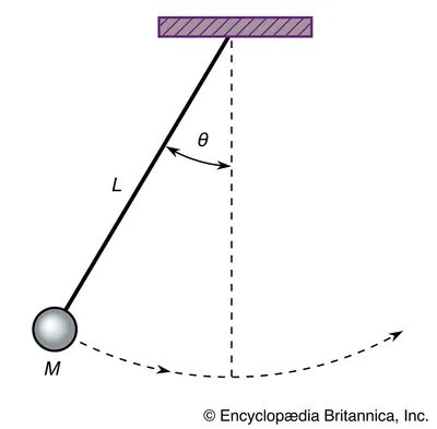
A massless rod of length is fixed to the ceiling with a mass on the end. The rod is subject to gravity and able to swing freely. Given a starting angular displacement , find a function that gives the angular displacement at time .

Deriving the Differential Equation

First, we use the laws of mechanics to derive a relation between and time derivatives of (, ). Then, we will solve for a that satisfies that relation.

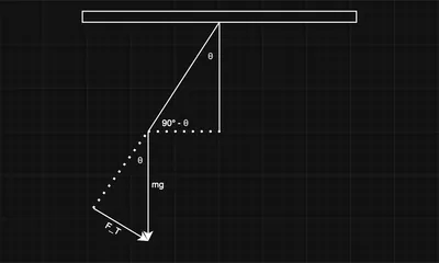
While the pendulum is displaced from the vertical, part of the downward gravitational force is acting on the pendulum tangent to its circular path. Using trigonometry, we can find the magnitude of the tangential component of the vector.

According to Newton’s Second Law of Motion, the absolute value of the force tangent to the path must be equal to mass, , multiplied by the absolute value of the acceleration tangent to the path.

Note that a symbol with a dot over it represents the time derivative of that value e.g. , .

, the displacement along the circular path from vertical, can be calculated from the angular displacement in radians, , and the length of the rod, .

Thus,

Eq. 6 tells us that the magnitude of the force acting along the path of the swinging mass will be equal to multiplied by the magnitude of the angular acceleration.

Should be equal to or the negation of in the context of the problem? Physics takes no prisoners, this must be right or everything downstream will be totally off.

Travel along the circular path is analogous to travel along the standard axis. Position, or , is positive right of center, negative left of center. Velocity, / , is positive insofar as / are increasing. Acceleration, / , is positive insofar / are increasing. On the right hand side where and are positive, the velocity starts positive and turns negative meaning acceleration is negative. On the left hand side where and are negative, the velocity starts negative and turns positive meaning acceleration is positive. Thus, we conclude should be the negation of .

We must find a that when differentiated twice with respect to time equals of itself.

As we’ll see, this is easier said than done. This difficult equation is often simplified by substituting for . This approximation is actually accurate for very small , leading it to be called the Small Angle Approximation.

Although I facetiously referred to this approximation as “heinous” in the introduction, it’s useful to go through the solution before dealing with the complexity introduced by in the exact equation.

Solving the Small Angle Approximated Pendulum Problem

The simplified differential equation.

We want to dump the second derivative on the left hand side through integration. If we were to naively integrate both sides of Eq. 12, it would maintain equality but would not be productive. Given that is unknown, is also unknown and cannot be evaluated. However, integration can be performed on an unknown function multiplied by its derivative via the reverse chain rule.

Multiply both sides by . Note that on the left hand side, this new term serves as the “base” and is the “chained” term.

Integrate both sides with respect to . This preserves equality.

is a constant of integration. Constants are removed by differentiation, so we can’t integrate without adding a constant to the equation. We can find here by leveraging our knowledge that the pendulum starts at rest at a known initial displacement, . We could carry through the rest of the steps and solve for it at the very end, it’s just easy to do so now.

Solve For based on initial conditions and .

Substitute the value into Eq. 15.

Solve for .

To integrate away this last , we need to do a separation of variables. We rearrange the and to be in expressions with only and respectively.

The integral can’t be evaluated using standard polynomial integration rules. We rely on a visual match to the integral definition of .

Click to See Derivation ▼

For

[a]

We want to show

[b]

Take the of both sides of Eq. A.

[c]

Take the derivative.

[d]

Invert both sides.

[e]

Substitute for .

[f]

Substitute for .

[g]

[h]

Solve for using initial condition .

Substitute for C and move it to the left hand side.

Take the the of both sides.

Simplify by substituting for .

Rearrange to find .

To Summarize, we

1. Used integration to turn and solved quickly for the first constant of integration using initial conditions
2. Separated variables to produce an equation of the form
3. Identified the integral on the right hand side to match the integral definition of
4. Substituted into the equation and solved for the second constant of integration
5. Took of both sides
6. Solved for

This approach is mirrored for the Non-Linear Differential Equation.

Solving the Non-Linear Differential Equation

We start with the exact pendulum differential equation.

Multiply both sides with .

Integrate both sides with respect to .

Find given initial conditions and .

Substitute the calculated value into Eq. 32.

Solve for .

Rearrange to separate variables.

Now we see why the Small Angle Approximation is so helpful. After the separation of variables, the integral exactly matched that of a well known function, . In this case, there are no obvious outs. Of course, the right hand side can’t be evaluated using standard integration rules. Instead, all we can do is marry it up to the integral definition of a known reversible function. The only way to proceed is through educated guess and check.

We hypothesize that we can algebraically manipulate the equation such that the integral on the right hand side matches that of . Upon success, we substitute for the integral and then take of both sides and be left with something looking like as the solution. There is no deterministic recipe for finding the right target function or the path to manipulate the equation in its direction.

The first guess (spoiler alert, it will work!) is , the inverse of the elliptic sine function. The integral definition is also called “The Incomplete Elliptic Integral of the First Kind.” From now on, that will be referred to as the IEIFK.

I’ve seen it written in two forms: Legendre’s Form

and Jacobi’s Form where and . and are arbitrary symbols.

We’ll use Legendre’s Form.

Note that is a constant value, also called the Elliptic modulus.

This is a reasonable guess for two reasons. First, elliptic sine is periodic which matches the observed behavior of the pendulum. Second, it’s not algebraically distant. After a substitution into Eq. 37 based on the half angle identity,

it’s closer but not an exact match.

is constant, so rename it to and multiply the to the left hand side to simplify the expressions in the following steps.

The denominator doesn’t match that of the IEIFK exactly. This doesn’t mean it’s game over, we just need to define a new variable, , through a relation to . If this relation allows us to marry up the right hand side of Eq. 42 to the IEIFK, we’re good. So long as we can calculate from , is a solution to the entire problem. To be useful, must be defined such that

Upon substitution into Eq. 42 the numerator will cancel out leaving the IEIFK with respect to .

Unfortunately, this is another educated guess and check. Steps toward simplicity are generally productive. Taking a look at the denominator, if we can change the to , then the denominator can be simplified to through the Pythagorean Identity.

Hypothesize .

Close, but then the numerator remains its ugly self. However, this attempt highlights another opportunity. If we take , the denominator can still be simplified through the above step.

Additionally, taking ( was defined right after Eq. 41), we can simplify the numerator as well.

Now we check the hypothesis by differentiating with respect to .

This matches the end of Eq. 47. Apply the simplifications from Eq. 46 and Eq. 47 in reverse.

To summarize this step, we derived via relation by “meeting in the middle.” The intuition for trying was that it simplified the numerator and denominator of Eq. 42. Once we differentiated directly we found that it satisfied the proportionality constraint with the constant factor, .

Substitute Eq. 51 into Eq. 42 remembering that we defined .

Integrate both sides. Definite integrals are needed to match the exact form of the IEIFK. This preserves equality.

Some insist on changing the variable inside the expression (e.g. and ) so it’s different from the integral upper limit ( and ). Eq. 53 may be improper or even “wrong”, but I find it easier to follow in this specific instance.

Substitute for the IEIFK.

Solve for using initial condition , remembering and .

For the sake of brevity, we’ll leave and continue from Eq. 54.

Take the of both sides.

Substitute for . Remember that is an invented variable without physical significance that we don’t want now that it has served its purpose of creating the IEIFK.

Solve for and note and .

Q.E.D.

To Summarize, we

1. Used integration to turn and solved quickly for the first constant of integration using initial conditions.
2. Separated variables to produce an equation of the form .
3. Identified that couldn’t be evaluated and manipulation would be needed to substitute for some . Nothing was an exact match off the bat.
4. Targeted the Incomplete Elliptic Integral of the First Kind for the right hand side due to the periodic nature of and algebraic proximity.
5. Made a substitution based on the half angle identity and then defined a new “utility” variable to get it to match up exactly.
6. Substituted and solved for the second constant of integration.
7. Took of both sides.
8. Solved for .
9. Used the relation between and defined in Step 5 to solve for .

Hopefully, this article made the Pendulum Problem less of a mystery.

Comparison of the Exact and Approximate Functions

For each frame, the pendulum position is calculated in your browser using the two functions derived above. For calculating and I used Claude to translate Cephes code to Typescript. This animation uses a positive 60 degree starting point, which is punishing for the Small Angle Approximation. I find the motion more robotic and less “real” in the approximated case. By contrast, the exact pendulum model shows slower motion close to 60 degrees.

Sources

Pendulums and Elliptic Integrals published in 2004 by James Crawford was extraordinarily helpful. I used the same algebraic path with some more explanatory notes and one minor error fixed. Crawford adds a lot of detail about numerical methods which I didn’t touch on here. It’s definitely worth a read if you’re interested in computation of and other algorithms for numerical integration.

I also studied Edmund Whittaker’s solution in Analytical Dynamics of Particles and Rigid Bodies. The old textbook has had pretty remarkable longevity given how much time I spent staring at it 122 years after publication. I found the content to be very thorough, even taking into account a pendulum which is given some starting speed*. It’s definitely worth a read if you are interested in “gloves off” Classical Mechanics.

*You then have to consider the case where the starting speed takes the pendulum over the top leading to two separate equations of motion.

James Crawford

Sir Edmund Taylor Whittaker

Thanks Boys 🫡